形態學運算（Morphological Operations）

形態學運算主要應用於二值影像，用來分析與處理影像中物件的形狀、結構與分布。相關功能集中於 Process > Binary > ...子選單中。

基本操作

Make Binary 建立二值圖：將影像轉換成黑白（0/255）圖像。預設會根據選取區域或整張影像的直方圖，自動決定閾值。若已設定閾值（Image > Adjust > Threshold），將會跳出對話框詢問設定前景/背景顏色，以及是否反轉黑白。
Convert to Mask 轉為遮罩：根據目前的閾值設定將影像轉成二值圖。若未設定閾值，則會自動計算。預設輸出為「反轉 LUT」（白為 0、黑為 255），除非在 Process > Binary > Options 中勾選了 Black Background。

侵蝕與膨脹（Erode & Dilate）

Erode 侵蝕：從黑色物件邊緣移除像素，相當於縮小物件。可用來去除尖角、毛刺或細小突出。對灰階影像可使用 Process > Filters > Minimum 模擬。
Dilate 膨脹：向黑色物件邊緣加入像素，相當於擴大物件。可填補小孔或斷裂。對灰階影像可使用 Process > Filters > Maximum 模擬。

組合操作

Open 開啟：先侵蝕再膨脹。可移除小雜訊、斷開細連線。適合清除背景雜點而不影響主體。
Close 關閉：先膨脹再侵蝕。可填補小孔洞、連接相近物體。適合使主體更為連貫。

其他操作

Skeletonize 骨架化：持續移除物體邊緣像素，直到只剩單像素寬的骨架。用於分析結構拓撲（如細胞通路）。
Outline 描邊：對物件產生單像素寬邊框。可視為邊緣檢測的一種形式。
Distance Map 距離變換：計算每個前景像素與最近背景像素的歐式距離，結果為灰階圖，產生Euclidian distance map (EDM)。適合用於分析粒子間距或後續分割。
Ultimate Points 終極點：對距離圖找出每個粒子內最大內切圓的中心，灰階值代表半徑。可作為分割粒子依據。產生ultimate eroded points (UEPs)。
Watershed 分水嶺分割：自動分離接觸或重疊的粒子。流程包含建立距離圖、找終極點，然後從終極點開始膨脹直到互相接觸為止。適用於圓形、不重疊太多的粒子分離。
Voronoi 沃羅諾伊分割：依據與最近兩個粒子的邊界距離，為每個粒子建立一個區域。適合做為粒子領域劃分（Voronoi tessellation）。

設定選項（Options）

透過 Process > Binary > Options... 可調整以下參數：

Iterations（次數）：設定侵蝕、膨脹、開啟、關閉等操作的重複次數。
Count（鄰近像素數）：決定侵蝕/膨脹時像素被加入/移除所需的鄰近像素數。
Black Background：勾選此選項代表背景為黑，物件為白。這會影響大多數形態操作與距離圖的計算。

可用下列方式設定：

    // Plugin
    Prefs.blackBackground = true;

    // Macro
    setOption("black background", true);

Pad Edges when Eroding：勾選時，侵蝕操作不會作用於影像邊緣（避免邊界損失）。
EDM Output（距離圖輸出格式）：設定 Distance Map、Ultimate Points、Voronoi 等輸出的格式：
- "Overwrite"：覆蓋原圖（8-bit）
- "8-bit" / "16-bit" / "32-bit"：輸出為新的影像，32-bit 為 subpixel 精度。

實作

幾何圖形

執行以下Macro，進行各種二值化操作，觀察這些圖形的變化

二值化影像

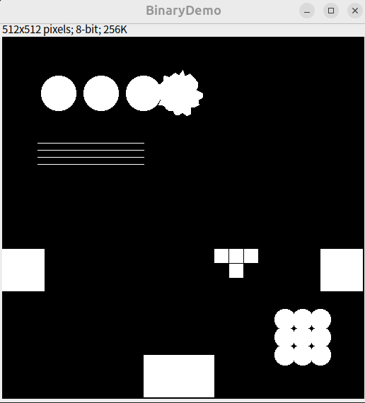
// 建立空白影像
newImage("BinaryDemo", "8-bit black", 512, 512, 1);
setForegroundColor(255, 255, 255);

// ---------- 粗圓 + 毛刺 ----------
for (i = 0; i < 3; i++) {
    x = 80 + i * 60;
    y = 80;
    r = 25;
    makeOval(x - r, y - r, r * 2, r * 2);
    fill();
}

// 毛刺圓形
centerX = 250;
centerY = 80;
nPoints = 36;
xPoints = newArray(nPoints);
yPoints = newArray(nPoints);
for (i = 0; i < nPoints; i++) {
    angle = 2 * PI * i / nPoints;
    r = 25 + random() * 10;
    xPoints[i] = centerX + r * cos(angle);
    yPoints[i] = centerY + r * sin(angle);
}
makeSelection("polygon", xPoints, yPoints); fill();

// ---------- 細線 ----------
for (i = 0; i < 4; i++) {
    y = 150 + i * 10;
    makeLine(50, y, 200, y);
    run("Draw", "slice");
}

// ---------- 貼邊形狀 ----------
makeRectangle(0, 300, 60, 60); fill();
makeRectangle(450, 300, 60, 60); fill();
makeRectangle(200, 450, 100, 60); fill();

// ---------- 破碎物件 ----------
setColor(255, 255, 255);
makeRectangle(300, 300, 20, 20); fill();
makeRectangle(321, 300, 20, 20); fill();
makeRectangle(342, 300, 20, 20); fill();
makeRectangle(321, 321, 20, 20); fill();

// ---------- 密集群圓 ----------
x0 = 400;
y0 = 400;
r = 15;
for (i = 0; i < 3; i++) {
    for (j = 0; j < 3; j++) {
        dx = x0 + i * 25;
        dy = y0 + j * 25;
        makeOval(dx - r, dy - r, r * 2, r * 2);
        fill();
    }
}

// 二值化
run("Make Binary");

細胞分佈

執行以下macro，產生三張圖片，模擬不同的粒子分佈，試試看執行Voronoi分隔。

// 參數設定
width = 512;
height = 512;
pointRadius = 3;

// 建立空白影像
newImage("Multi-Pattern Particles", "8-bit black", width, height, 1);
setForegroundColor(255, 255, 255);

// -------------------- 區域1：隨機分佈 --------------------
nRandom = 50;
for (i = 0; i < nRandom; i++) {
    x = random()*160 + 10;    // 區域X: [10,170]
    y = random()*160 + 10;    // 區域Y: [10,170]
    makeOval(x - pointRadius, y - pointRadius, pointRadius*2, pointRadius*2);
    fill();
}

// -------------------- 區域2：密集群聚 --------------------
nClusters = 3;
pointsPerCluster = 20;
for (c = 0; c < nClusters; c++) {
    cx = 200 + c * 30 + random()*10; // 區域X: 約在 200-300
    cy = 60 + random()*60;
    for (i = 0; i < pointsPerCluster; i++) {
        dx = random()*20 - 10;
        dy = random()*20 - 10;
        x = cx + dx;
        y = cy + dy;
        makeOval(x - pointRadius, y - pointRadius, pointRadius*2, pointRadius*2);
        fill();
    }
}

// -------------------- 區域3：規則排列 --------------------
for (i = 0; i < 6; i++) {
    for (j = 0; j < 6; j++) {
        x = 350 + i * 20;
        y = 50 + j * 20;
        makeOval(x - pointRadius, y - pointRadius, pointRadius*2, pointRadius*2);
        fill();
    }
}

// 完成後進行二值化
run("Make Binary");

Top-hat 濾波

Top-hat 濾波是一種基於形態學開運算的背景校正與特徵增強方法，分為： - 白 Top-hat：原圖 - 開運算結果，突顯比結構元素小的亮特徵（常用）。 - 黑 Top-hat：閉運算結果 - 原圖，突顯比結構元素小的暗特徵。

主要應用

背景分離/校正：移除不均勻照明、背景雜訊，讓前景物體更明顯。
對比增強：提升小型亮（或暗）特徵的對比度。
特徵提取：強調影像中特定大小的細節，便於後續分割或量測。

ImageJ 操作

Process > Filters > Top Hat...

結構元素半徑建議大於目標特徵，且小於背景變化尺度。

Macro 範例

run("Blobs (25K)");
run("Invert LUT");
run("Duplicate...", "title=topHat50");
run("Top Hat...", "radius=50");

回到首頁